There are several federal web services that are currently providing geospatial data that is essential for your design projects. As a civil engineer that specializes in hydrologic and hydraulic design, I need to know the watershed delineation for the site as well as the limits of the FEMA regulated floodplains.
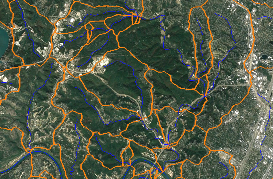
For watershed delineations, the EPA WATER's service (Watershed Assessment, Tracking & Environmental Results System) provides for the request and delivery of pre-calculated watersheds and stream centerlines for the continental United States.
When you need FEMA floodplain limits on and adjacent to your subject site, most folks these days use FEMA's National Flood Hazard Layer (NFHL). Typically, this is ingested through an image overlay map service that is used in either Google Earth, ArcGIS Pro or QGIS.
Dynamo: Getting AutoCAD Linework
I have created a couple of Dynamo scripts that makes a web request to these federal servers to get the needed AutoCAD linework for your drawing. Here is a rough breakdown of what is going on:
User sets up a Civil3D drawing in the desired Coordinate Reference System (CRS)
User draws and selects ACAD item for spatial input
Dynamo converts items coordinates to Latitude/Longitude
Dynamo builds a URL to request the data from the REST endpoint as JSON
Prior to even thinking about using this script, you will need to install the Civil3DToolkit package for Dynamo. This package is provided by Autodesk and provides functionality necessary for my scripts to work.
Download the Script
Download the Civil3D Dynamo scripts from my GitHub repository.
The scripts are "as is" and are provided without warranty of any kind. You can modify any script but, if you do, know that you are required to provide me proper credit.
Please comment below if you have questions or issues. While I can't provide support, I would like to know what issues y'all are seeing.
When using pipe networks in Civil3D, the civil designer is always required to determine if (1) pipes are not clashing with each other and (2) if the pipes have the appropriate [and often statutory] minimum vertical clearance. In municipalities that I have designed projects, this minimum vertical clearance between the outside diameters of the pipes is 2 feet (24 inches).
So....
You have designed all of your pipe networks both horizontally and vertically. Some of these are gravity networks (storm drain, waste water) and some of these networks are pressure (water, force mains).
Using Dynamo for Civil3D, I am providing you a FREE tool to evaluate all the pipe crossings provide the minimum vertical clearance.
Stop (Collaborate and Listen)!
Prior to even thinking about using this script, you will need to install the Civil3DToolkit package for Dyanmo. This package is provided by Autodesk and provides functionality necessary for my script to work.
Download the Script
Download the Civil3D Dynamo script from my GitHub repository.
The script is "as is" and is provided without warranty of any kind. You can modify the script but, if you do, know that you are required to provide me proper credit.
1) I have noted that some alignments may not be properly processed. If that is a problem, place all alignments on the same layer or move the alignments to a '0' layer.
2) DO NOT run the script in 'Automatic' mode. The creation of a new pipe in automatic mode will likely crash Civil3D.
3) Set the Layer color to "ByLayer" prior to running.
Please comment below if you have questions or issues. While I can't provide support, I would like to know what issues y'all are seeing.
When it comes to bridge modeling in HEC-RAS, there are a few items that you need to take into consideration:
Station Control: All bridges inside of HEC-RAS are a based upon a alignment layout. Think of it like a cross section. You have a horizontal alignment where a station (X value) has a corresponding elevation (Z value).
Bounding Cross Sections:Cross sections both upstream and downstream of the structure to be modeled are necessary. To make modeling easier, it is recommended that both of these cross sections be the same length and therefore have the same station control.
High Chord: The 'high chord' is the top of the bridge to be modeled. For an existing bridge, often LiDAR is available to help model these station-elevation pairs, which is typically the roadway elevation, rail road or other similar item. Sometimes the high chord should be modeled to include a concrete barrier, hand rail or metal beam guardrail.
Low Chord: The 'low chord' is the bottom of the bridge. These are station-elevation pairs modeled together with the high-chord. Often the low chord represents the bottom of the girder section or the bottom of the I-beams.
Piers:Between each bridge span a pier can be modeled. These are entered along the station control at width-elevation pairs. I typically model the piers at an elevation of zero and ending at an elevation between the high and low chord. Often the bents capping the piers are wider than the piers and are modeled as part of the pier.
Abutments: At the end of bridge span, bridges have abutments. If this abutment is vertical it can be modeled with geometric points of the low chord. It the abutment is sloping, it can be modeled in HEC-RAS with station elevation-pairs along the control alignment. This is done to make sure that the conveyance (flow) area under the bridge is correctly modeled.
Ineffective Flow Areas As water flows though a bridge, it accelerates and funnels into to area under the bridge. As water flows out from under a bridge, the water spreads out and expands back into the full conveyance area of the floodplain. While water moves quickly through the bridge opening, areas of the upstream and downstream bounding cross sections that are not adjacent to the bridge opening may be wet but have little to no velocity or conveyance. Around a bridge, it is necessary to model ineffective flow areas so that HEC-RAS knows areas that are likely to get wet but have no velocity or flood conveyance.
A video tutorial
Wow! It seems like there are several items to manage when modeling a bridge. How to keep all of them straight? I have added a video that walks through the whole bridge modeling process. Enjoy.
For every civil engineering project, there must be topographic terrain data for the site. In the early days of my career, I would have to twiddle my thumbs waiting for the surveyors to the field acquire the required survey shots. No work could commence until I got their survey and built an existing ground surface model.
Now, LiDAR flights are made regularly throughout the United States scanning the landscape. With my work currently focused in Texas, I am always on the 'hunt' for current terrain data whether it is for a small site or a large drainage study.
Texas now has LiDAR coverage for the entire state. While some data are in processing, I suspect that within a year (2021) Texas will have complete coverage served via the Texas Natural Resource Information Service. (TNRIS)
There are multiple flights, thousands of tiles and petabytes of data in the form of both bare earth terrain digital elevation models (DEM) and LiDAR point clouds (LAS). For every project the task is to:
Determine which tiles are needed for the project
Downloading and unzipping the tiles
Merging the tiles into one (1) single DEM
If needed, clipping the terrain to the requested boundary limits
Wouldn't it be awesome if this entire process could be automated? This is what I accomplished via a Python script.
All the files needed to replicate this workflow on your machine are at GitHub.
First, we must create an ESRI shapefile of the requested area. For this example, we are going to grab the entire limits of the Walnut Creek watershed in Austin, Texas. We will use polygon (area) shapefile named "Walnut_AOI_AR_2277.shp". Note that this file is in EPSG: 2277 (Texas Central State Plane, US ft).
Via the Python code, this shapefile is translated with GDAL and intersected with a TNRIS provided tile index shapefile (EPSG: 4629). A list of the required tiles is returned and URLs are programmatically constructed to prepare for downloading.
Inputs needed:
Quarter Quad Index - StratMap_QQ_Index_AR_4269.shp
Texas available tiles - TNRIS_LiDAR_Available_AR_4269.shp
Note that for this example, ten (10) quarter quadrangles (QQ) will be downloaded to cover the requested area. When unzipped, each QQ contained sixteen (16) quarter-quarter-quarter-quads (QQQQ). We will need 79 tiles (QQQQ) to cover the area. [These counts assume no buffer]
Step 2: Download the Tiles
TNRIS allows download of bare earth LiDAR DEMs through an Amazon Web Service (AWS). Here is an example URL of one (1) of the QQ tiles.
This is for one of the tiles in the 'stratmap-2017-50cm-central-texas' data bucket on AWS. Using multi-threading, the routine downloads multiple tiles (QQ) at once using the Python requests library. Still... download speeds may vary. After unzipped, this is 911 Mb of data.
Step 3: Merge the Tiles
Using the Python 'rasterio' library, the downloaded tiles are filtered to those QQQQ tiles within the requested boundary. All other tiles (QQQQ) are deleted. Then the remaining tiles are merged into a single DEM.
Step 4: Clip and Re-project
Finally, the merged raster is clipped to the requested boundary limits (plus a buffer). This DEM is projected to the same coordinate system of the requested boundary shapefile. For this example it was EPSG: 2277 (Texas Central State Plane- US foot)
What is needed... Anaconda + Environment
To use this routine on your own machine you will need to do the following.
Open the anaconda command prompt. In the Start menu, type in 'Anaconda' and select the Anaconda Prompt (Anaconda3) application.
My machine is named FN34GZ1. Your path will definitely be to a different location.
Copy the GitHub provided specifications file (terrainharvest_speclist.txt) to the same folder seen in the anaconda command prompt. (Mine is 'C:\Users\FN34GZ1')
In the anaconda command line, create the 'harvest' environment by entering in the following command.
After installation is complete, activate the 'harvest' environment
conda activate harvest
Notice that the environment changed from 'base' to 'harvest'. That means that the 'harvest' anaconda environment is now active.
With the 'harvest' environment active, launch jupyter notebook from the command prompt.
jupyter notebook
This will open Jupyter Notebook... which runs inside of a web browser.
Jupyter Notebook
Copy the 'TNRIS_Terrain_Harvest.ipynb' notebook from the GitHub resource to a folder named 'Terrain_Harverst' under the anaconda root directory. My location is 'C:\Users\FN34GZ1\Terarin_Harvest'. Your path will vary.
In Jupyter, select the folder that you created.
Select and open the file named 'TNRIS_Terrain_Harvest.ipynb'.
This notebook script needs to run with the 'harvest' environment that was previously created. In Jupyter --- change the kernel to 'Python [conda env: harvest]'
Jupyter Notebook - Inputs and Outputs
There are three (3) input shapefiles that are needed to run this notebook. The first two are indices of the TNRIS tile scheme. The third shapefile is a requested boundary of the area needed. All of these shapefiles must be polygons. The requested boundary will only utilize the first found polygon. You can not request multiple areas at once.
Revise the path to the tile indices in the "2.0 Input Data" code block. Revise the path to the requested boundary shapefile.
Change the output directory to a location that exists on your machine.
Jupyter Notebook - Run the Notebook
To run the notebook, under the kernel menu, select the "Restart & Run All". Provided the size of the request and the speed of your internet connection, the procedure could take several minutes.
Ultimately, the routine returns a merged DEM whose units are native to the tiles that are served by TNRIS. This means that the completed tile is likely in UTM and the vertical data is is meters.
Courtesy of the maestro, Paolo Serra of Autodesk, the Civil3D team has been furiously working on improvements and additions to the dynamo interface via the Civil3DToolkit. With a standard install of 2021, dynamo is currently limited to interfacing with alignments, points, corridors and surfaces.
The addition to the dynamo tools expands the ability to interact with parcels, sites and feature lines within your Civil3D drawing. Their revised toolkit also provides dynamo node exposure to gravity pipe networks and pressure pipe networks.
I recently (21 Sept 2020) installed Civil3DTollkit 1.1.10 to see how quickly a novice could ramp up on the new tools. Here are a items that I quickly discovered regarding dynamo in Civil3D:
As we typically work in State Plane with large coordinates, ensure that "Extra large" geometry working range is selected before creating your own or executing someone else's dynamo script.
Have a basic understanding how lists work as many requested dynamo nodes will output a list. In most programming languages, the first item in the list is provided an "index" of zero and the counting commences from there. Here is a quick into to lists.
Knowing a little bit of Python coding doesn't hurt. You can write a quick script if needed to solve problems where a provided nodes just doesn't do it.
Dynamo has it's own geometry language that differs from Civil3D and AutoCAD. Often to accomplish your goal, objects will have to be converted. For Example... Civil3D alignments may have to be converted into Dynamo PolyCurves to use some dynamo provided tools.
Carve out some time and begin your experimenting. Before you begin... all Civil3D users should install the latest Civil3DToolkit. This is a package that you we need to get access to the latest Civil3D nodes.
My first working example (note the "Add-ons" from the Civil3DToolkit):